Like yours, my pool cleaner is on the output side of the pump, and every ~5 mins its reverse thruster valve opens. That picks it up and dumps it somewhere else in the pool. That’s enough of a change in flow rates to show up at the energy monitor as a ~15W divot.
dBC, wow, I hadn’t even considered those traces being from your energy monitor, but it makes sense.
If I am understanding correctly, that long trace is made up of continuous sampling/calculating for 10 seconds at a time. So, even though the graph is shown as a continuous line, it really is made up of discrete points (reported every 10 seconds) connected by the graphing program.
I’m trying to figure out exactly what information I want to get/characterize (in my project) and it comes down to this. I want to see what impact my (eventual) changes to my pool’s cleaning system does to my pump’s Energy Factor, which is calculated as (1000s of gallons pumped per kWh).
I won’t necessarily need 10-second chunks of power, especially considering I might not have the corresponding 10-second chunks of pump GPM that correspond to that power. Whatever I end up collecting (GPM & wattage)I will be accumulated and averaged over one (or more) complete zone of my pool’s cleaning system (about 5 minutes) in order to compare it to my sytem’s “pre-change” Energy Factor.
I agree that the trace from your pool will be closer to my pump’s operation, but I expect there to be larger variations in the wattage and GPM on my cleaning system. Typically my IFCS runs about 800 watts at the plateaus (in my previous diagram). In the valleys, I expect that to go up as high as 1100 watts.
Actually, the same is true of the scope-like per-cycle trace, but in that case the datapoints are every 250 usecs. In the latest version of that energy monitor they’re every 125 usecs (8 kHz is the fundamental beat of the energy IC), but that one is still on the bench in the lab so I couldn’t easily point it at my pool pump or washing machine.
I have been doing some testing with my new “sketch”. I have some more planned but wanted to check if I am off base on a couple assumptions. As it turns out, a dedicated Photon seems to be very capable of doing the real-time calculations necessary for continuous power measurements. I still haven’t dragged the setup out to my pool pad area, but I am getting close.
In this code posting, I have stripped down the code to a minimum (NO multi-cycle summing/averaging, etc). This code just takes a SINGLE cycle of data at a time and reports the power. Surprising to me, for all my “lab testing” including crock pots, hair dryer, floor fan…the power reading matches the Watts Meter within ~1% for all cases except at the very low end…with just a SINGLE CYCLE of sampling. Obviously these “lab loads” must be very regular, including the small motor devices that I am testing.
(1) So after talking me out of using “Apparent Power” as “good enough” (thanks to the knowledge/advice of all those that have helped), I have moved toward the opposite extreme: what good is Apparent Power? For use cases such as mine, is there an advantage to calculating RMS Voltage, RMS Current, power factor rather than going straight to the Real Power number?
(2) Also, I assumed (probably incorrectly) that the voltage and current offsets (due to the DC biasing of the sampling circuits), could be calculated/measured one time and then used exclusively as a constant…that’s shown in my “sketch”. I assumed that these values would be based on the actual resistances of the voltage dividers implemented, which I wouldn’t expect to change that much. It’s worked well the last couple days, but today they are off from my previous measurement. Is that variance “expected” and the reason why these offsets are calculated dynamically? Or did I just bump my breadboard?
Anywhere, here is the “sketch”…probably the only thing of interest for those following this, is the ISR routine itself which “calculates” the instantaneous power (Sample_ISR). In this minimized code, the sample rate is 333uSec (50 samples/cycle @ x60mHzx 60Hz).
#include "SparkIntervalTimer.h"

#define PUBLISH_TIME 2000        // 1000ms = every second
#define FREQUENCY 60             // 60 = 60Hz, 50 = 50Hz
#define SAMPLES_PER_CYCLE 50
#define ISR_SAMPLE_INTERVAL (int) (1000000/(FREQUENCY*SAMPLES_PER_CYCLE))  // in uSec
// The following constant is experimentally determined using a watts meter
//    = (Power Reading on Watts Meter) / power_uncalibrated
// eliminates need to use/calculate RMS voltage/current
#define POWER_CALIBRATION_CONSTANT  7.804232804232804e-4

IntervalTimer myTimer;

volatile long power_uncalibrated;
unsigned long currentMillis, prior_publish_time;
bool timer_started = false;
volatile bool sample_is_complete = false;

//Forward Function Declaration
void Sample_ISR(void);

void setup() {
  pinMode(D7, OUTPUT);  //BUG: required to enable the interrupt/IntervalTimer function...BUG on the PHOTON
  setADCSampleTime(ADC_SampleTime_144Cycles);  // Approx Conversion Times: 480=80us, 144=27us, 84=14us
}

void loop() {
  currentMillis = millis();

//Setup the ISR Current & Voltage Sampling Rate
  if (!timer_started) {
    myTimer.begin(Sample_ISR, ISR_SAMPLE_INTERVAL, uSec, TIMER7);
    timer_started = true;
  }

// Print the latest available power values every PUBLISH_TIME
  if (sample_is_complete && ((currentMillis - prior_publish_time) >= PUBLISH_TIME)) {
    Serial.printlnf("Power: %.1f Watts   sTime: %.2fms   power(raw): %d", power_uncalibrated * POWER_CALIBRATION_CONSTANT, (ISR_SAMPLE_INTERVAL/1000.0), power_uncalibrated);
    prior_publish_time = currentMillis;
    sample_is_complete = false;
  }

}


void Sample_ISR(void) {

#define VOLTAGE_OFFSET 2034   // previously measured offset
#define CURRENT_OFFSET 2018   // previously measured offset
static long sumP;
static uint32_t sample_counter = 0;
int16_t i_sample, v_sample;

  if (!sample_is_complete) {
    i_sample = analogRead(A0)-CURRENT_OFFSET;
    v_sample = analogRead(A1)-VOLTAGE_OFFSET;
    sumP += v_sample * i_sample;      //Sum the instantaneous power
    sample_counter++;
  }

  if (sample_counter >= SAMPLES_PER_CYCLE) {
    power_uncalibrated = sumP/sample_counter;
    sample_counter = 0;
    sumP = 0;
    sample_is_complete = true;
  }
}
SAMPLE OUTPUT from this sketch (prints instantaneous power every 2 seconds)
This looks promising - I think you’re on the right track.
It’s a measure of the power you are apparently drawing if you measure voltage and current separately (using an ordinary multimeter, say) and multiply the readings. Hence the name.
It relates to power factor, which should be on the pump’s label, and hence to current, hence to the wire size, switch ratings etc you need to use. A poor power factor means higher current and so a bigger wire size, and the poor power factor means the load is highly inductive (or capacitive), which reflects on the rating of the switches you need to control it - a switch rated at say 10 A resistive might be only 2 A inductive.
Or in terms of relating to what your supplier charges you - not a lot.
Indeed it is. Though you can expect both resistors to drift by about the same percentage, there’s no guarantee of that.
60 milliHertz ? an attack of digitus erroneous?
I note you’re using the calculated sample rate and count to determine what a cycle is. That will be OK if the frequency is tightly controlled where you are, and you’re only measuring over 1 cycle. In the UK, it’s guaranteed only within ±1%, so over 10 cycles we could be 5 sample pairs out - quite significant, which is why we are worried about the ‘end effect’ I mentioned earlier.
I presume that because your load is fluctuating, you’ll sample your one cycle fairly often.
I also see you’re not trying to take account of the phase and timing errors except as part of your overall calibration - phase errors coming from the current and voltage transformers, and timing from reading the voltage and current one after the other. If you calculate power factor, you could well find that swapping the order of reading will make a difference - in which case you need to get the power factor closest to unity with a pure resistance as your load. In emonLib and emonLibCM, we interpolate between successive voltage samples to apply the correction. You can expect the power factor to vary according to the load on the pump.
At the cost of accumulating the raw samples separately, you can correct the offsets after the event - calculate the average voltage and current for your 1 cycle (to give you the average error in each offset) then subtract the “offset power” from sumP.
Robert, thanks for the reply…wow, there is a lot of information in that post!
Yes, haha…edited…I have been thinking in mSecs quite a bit.
I am going to see how my testing/characterization goes…For my purposes, I am hoping to ignore this frequency variation completely, . But, you will see that errors could compound based on my plans below (measuring over multiple cycles).
My goal is continuous (at whatever discrete minimum sample rate I end up with), but that will require some changes. I don’t want to overload my existing pool controller firmware with too many interrupts. I could implement a “fast/accurate” mode and ONLY use it during my characterization process. But, I’d rather keep it “on” all the time, if it turns out to give me “enough” accuracy…TBD.
Some of that was planned (ignoring the sample time differences between the v & I), some of my choices are through blind ignorance. Besides my pool pump, I am also planning on monitoring the power of my Stenner pumps (only one is on at a time). So I am keeping the other side of my voltage sample “free” so that I can sample the Stenner current on the other side (voltage sandwiched between the two current measurements). But as part of my efforts, I will definitely swap the order to see what impact it may have on accuracy, as you have suggested.
The Particle.io Photon’s implementation of analogRead() is interesting. It has 10-bit accuracy (which I probably don’t need), and in firmware it actually takes 5 successive adc readings and averages them to give the user the end result. The default, and most accurate, sample time for each of those adc readings is 480cycles (I don’t know the frequency), and that translates to an execution time of 80uSec for the analogRead(). To this point I have been running at a sample time of 144cycle/adc sample…which corresponds to about 27uSec execution time for analogRead(). It can go even faster, and I may test some of those values. I assume that lower execution time for the analogRead()s translate to less phase differential in the v/i readings.
Good idea, and I will look into this a bit later…partly because I want to explore this idea a bit more first:
I have tested a fair amount on an earlier idea I approached you with: spreading out samples over multiple cycles but still based on the discrete times associated with sampling over one cycle. Intuitively, it just makes a lot of sense to me…and with my simple resistive loads/hair dryer/floor fan testing, it has been as accurate as taking all the samples over a single cycle.
I realize that a relatively “quick” changing load (my pool pump during IFCS operation) is the situation that is going to stress this approach. So I am going to setup up some firmware monitors to see how much accuracy is lost by doing it.
Like my (50_samples/1_cycle testing), the power readings for (50-samples/1_distributed_cycle) were within ~1% of actual for all my simple test cases.
Possible Sample Rates for 60Hz & 50 samples/“cycle”
333 uSec, 50 samples are taken across 1 cycle
1 mSec, 50 samples are taken across 3 successive cycles
3 mSec, 50 samples are taken across 9 successive cycles
9 mSec, 50 samples are taken across 27 successive cycles
27 mSec, 50 samples are taken across 81 successive cycles
There are also more scattered in between some of those (most, but not all odd numbers such as 7ms, 11mSec, 13mSec, 17mSecs, more)
For all but the last (27mSec), the accuracy of using these various sample times was undifferentiated through my manual readings. But I want to implement some in-program checks before I test my pool pump so that I can be more accurate in my assessment. Based on the numbers I get from my pool pump, I obviously would choose the lowest sample rate that I think I need for my purpose.
Anyway, that’s where I am headed for a bit. I hope it makes sense.
Bill, that is nice to know that maybe I don’t have to worry about the frequency drift! Also, thanks for pointing out that post/thread. I missed that thread in my searches but a lot of that discussion applies here. I wish I had seen it earlier.
Out of curiosity, is there a way in this board’s options to “line through” deleted text? Like bold or italicize but a line through it. I don’t see that option but I have seen it on other boards.
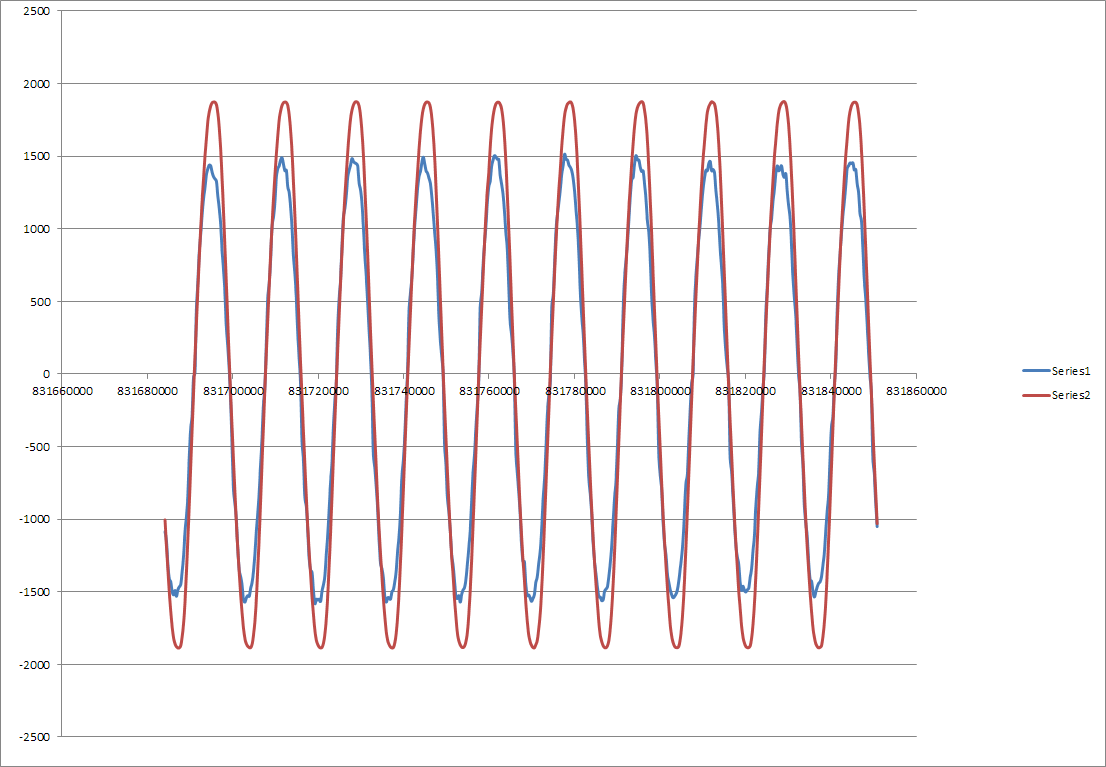
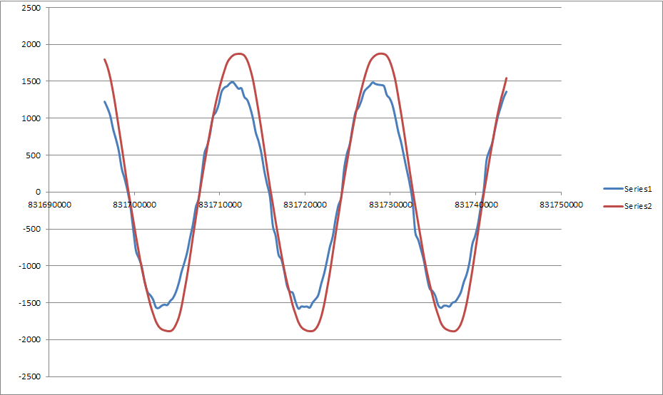
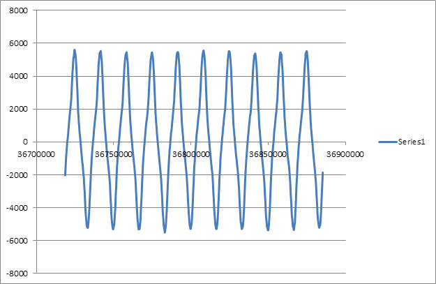
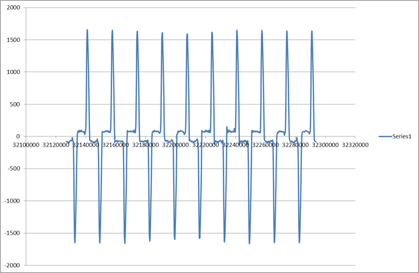
A couple graphs…it was painful, but I dragged my setup out to my pool pad just to see what kind of “current” waveform my Variable Speed Pool Pump produces. I recorded a few 500 point (10 cycle) graphs to see if there was anything unusual like with dBC’s washing machine. With these limited windows, I didn’t detect anything unusual…but I could have missed them.
The blue is the current…I multiplied my current by 5 in Excel because I am still currently using that 20amp SCT-013 and in this case I only threaded one wire through the loop for this check, the actual peak-to-peak was much smaller. No real numbers here and my calibration is not right (I think I need to multiply by 2 for the 220) and I still haven’t made code changes for the voltage/current offsets. Remember that by skipping the RMS calculations, I won’t have real voltage or current numbers. The graph timeline is in uSecs.
I hate it when underlying layers do that. They were probably trying to solve some problem with that, but there may have been better solutions. Is there anyway you can turn that off? It would be better if you were in control of how you space your sampling, rather than have it occur in clumps of 5.
I’m not familiar with the Photon but I am familiar with the underlying cpu they use (or at least closely related ones from the same vendor), and I recognise those numbers (480 cycles, 144 cycles etc.). I’ve just pulled up the GUI configurator for the part they use:
That “Samping Time” setting is how long the ADC’s S&H cap will be connected to your signal, after that time it disconnects the input pin from the S&H cap and commences the conversion, which takes an additional 13 cycles for 10-bit resolution.
So “more cycles → better accuracy” is not really true(*) - although I could believe that’s what the Photon doco claims. It’s pretty much a binary thing… either you’ve allowed enough cycles to fully charge the S&H cap from your signal source or you haven’t. How many cycles you need for that depends on the source impedance of your signal. Once you have that covered, increasing the samping time won’t improve accuracy. Conversely, if you don’t allow enough cycles to charge the S&H cap then you’re not operating the ADC as intended and all bets are off. So the aim is to set that parameter big enough, but no bigger.
The ADC maths for the numbers you quoted are:
(480 + 13) x 5 = 2465 cycles taking 80 usecs => 30.8 MHz ADC clock
(144 + 13) x 5 = 785 cycles taking 27 usecs => 29 MHz ADC clock.
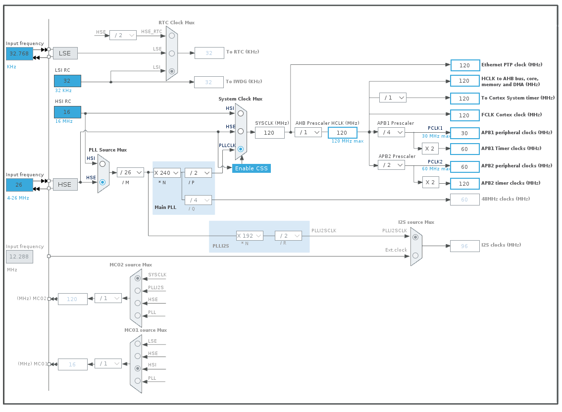
I pulled up STM’s clock configurator for the part they use, and I saw in the Photon docs they use an external 26 MHz crystal. So assuming they run the core at 120MHz I’m guessing their clock config looks something like:
which gives a PCLK2 of 60 MHz, and you can see in the ADC configurator above the ADC clock is PCLK2/2, which is 30 MHz… a very good correlation with your timings above. So I think you can safely assume your ADC clock is running at 30 MHz.
(*) EDIT - actually, if you’re measuring a noisy signal, a longer than otherwise necessary sampling period might help smooth things out by effectively using the S&H cap as your LPF, but there are potentially better ways to do that.
That’s very promising. Did you try different speeds? The more you know about how that waveform looks, the better informed you’ll be about how well any measurement shortcuts you take will perform. If it’s a nice sinewave under all conditions it gives you a lot of options not available to those of us trying to measure arbitrary current waveforms.
There is a way to do that…Particle.io has an open OS. But I’ve looked at a couple examples that make calls to the firmware and the code is very confusing to me, haha. Object Oriented Programming/Classes/etc are steps beyond my “easy to read” & understand concepts…if I need to do it, I probably could, but I’m in a test and see approach at the moment. I’d prefer to stick with the “user” instructions.
Thanks for figuring all that out. I have only seen the numbers “batted around” over on the Particle.io forum and was never positive that they were legitimate. It’s good to know that there is some basis in reality. You know your A2Ds!
Let’s see how my next set of “experiments” come out. I’m going to fiddle with the sampling rate, different values for the ADC’s S&H, averaging periods. Based on the data so far, I don’t think I’ll run in to any roadblocks to find something I’m happy with, but we will see.
Darn…didn’t see this note until after I dragged my setup back in. The problem is that currently, I have no way to grab data from my “test Photon” without a computer directly connected to it. That will change soon.
I only tested a few spots while my In-Floor-Cleaning-System (IFCS) was running at high RPM. I don’t expect to have any problems getting good power numbers at other times because everything in the system runs at a steady state during non-IFCS operation. BUT, I didn’t think about the fact that there still might be some interesting waveforms when the VSP pump is running at low RPMs.
I’ve been doing some experiments. When I started this project and was using the “somewhat flawed peak-to-peak Apparent Power” measurements, I noticed that for resistive loads (apparent power = real power), I could get pretty accurate measurements using that peak-to-peak strategy…even when my sampling was on the order of only a couple samples per second…but only if those sample were made at very specific timings…kind of like @Robert.Wall described in his post a few back (4 samples per cycle)…but spread out over many, many more cycles:
When @dBC showed some of the waveforms we might expect to see on some household appliances, I understood the problem that the experienced posters on this board were pointing out to me in regards to relying on a nice sine wave to calculate the RMS current using the .707 multiplier from peak-to-peak samples. But, I still believed that these ( I*V) readings could be obtained/summed with low frequency sampling, as long as the “timing requirements” for those samples are met. That’s what I have been playing with, and at least for what I have been checking, it seems to be working.
I don’t know the technical terms for this process, but I am sure it must be a standard technique in signal processing…and I am also sure that probably everyone else here understands it better than I do.
Anyway, when I looked at some of those weird current profiles that dBC has posted (and worried that my pool pump might be similar because it’s a VSP), I wondered what kind of sampling would be necessary to accurately capture those waveforms: 10 samples/cycle?…not likely…but I get the impression that 50 samples/cycle is an accepted number that gives accurate power readings. Now, how to spread those 50 sample points across multiple cycles so that it is infinitely repeatable/continuous.
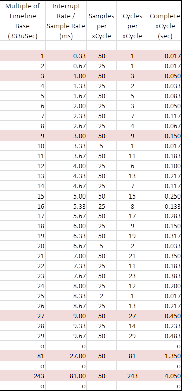
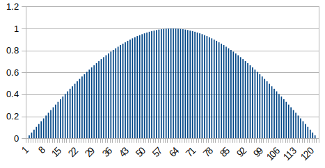
Given any frequency (50Hz or 60Hz in my case), and a “single cycle sample rate” that evenly divides into that frequency, there seems to be only ONE solution for each multiple of that “single cycle sample rate” to accomplish this purpose.
This chart is an example for a 60Hz frequency in which the fastest sample rate is 333uSec (50 samples/cycle).
In the above graph, the 2nd column gives the sample rate (sample every ‘x’ mSec)
xCycle refers to an extended Cycle, this is a term I made up because I don’t know what else to call it…“Cycles per xCycle” refers to the number of actual (60hz) cycles it takes to complete an xCycle and complete the sample count.
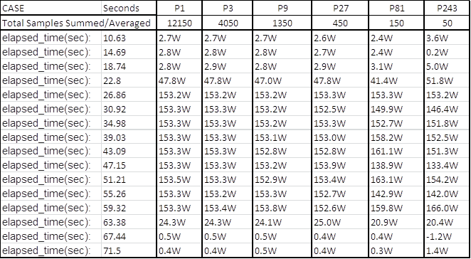
I did simultaneous tests at six different sample rates. They are highlighted in RED. At the slowest level (index = 243), the samples were taken every 81mSec. To “complete” its xCycle of 50 samples, it actually takes 4.05 seconds of time. I wanted to compare the accuracy of the results for all six cases. I didn’t choose these sample rates because they were the “best”, I chose them because they were easy and represent a wide range of possibilities.
Nobody probably cares about test cases on resistive loads…that is just too easy and too consistent. So I found a couple special case “appliances” to run these on. One is an air compressor that draws about 1000 Watts, I figured that is about as close as I am going to get to my pool pump . According to my Watts-Meter, the Power Factor is about .91 or so and it has a sawtooth current profile. The other is my DeWalt battery charger…it has a current profile similar to some of the ones that @dBC posted, you’ll see the picture.
In the program, the Power reported for each case is averaged over the longest period (4.05 seconds). Once again, this was just convenient and is not what I will end up with for my project. So in the first case, 50 samples are taken EVERY cycle (every 333uSec). These power numbers were then summed and averaged over the 243 complete cycles (4.05 seconds).
For the case of the 1mSec samples, there were 81 complete xCycles completed (0.5 mSecs each)…the power numbers were summed and then divided by 81 to report the average power for the 4.05sec period.
For the case of the 27mSec samples, there were ‘3’ complete xCycles completed (1.35 secs each), summed and averaged (divide by only 3) for its power average.
The last case (81mSec) is not averaged at all. It is purely the reporting of the power for the 50 samples taken over the 4.05 second period. Just one complete “xCycle”.
Here is the “current” profile for my air compressor. The results will show that the power requirements continually increase as the compressor has to work harder to “fill the the tank”. This graph doesn’t necessarily show that because it is only 10 cycles at 16.67mSecs each. But my sketch’s output will show the power increasing.
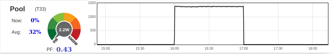
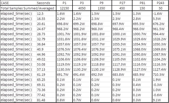
Here is the power reporting for all six cases (333uSec/sample to 81mSecs/sample) that I described in the last post. The timeline is on the left. During this test, I started out with no current and then turned on the compressor. You can see that even though I turned on the compressor mid 4.05sec sample, ALL the measurements account for it, even the case that is not averaged and only has 50 samples total (P243).
I let the compressor run for a number of seconds. The power continued to rise as the compressor increased it’s tank pressure. Then, you can see that I turned it off.
The other example will have to wait, my grandkids are up, haha.
So before I rerun that other example and record the results, here are a few comments. Most of these concepts are all new to me, and some of my thinking could be way off base…so feel free to burst my bubble.
A look at my numbers indicates that for the examples I have run, there is no need to sample 30-60 times a cycle to get an accurate power number. In fact, the P27 column indicates that with as little under 2 samples per cycle, an accurate power profile can be obtained. It’s even possible that the P81 (1 sample per 1.5 cycles) and P243 (1 sample per 5 cycles) columns will converge as well given a few more xCycles to average. As I said previously, these numbers were chosen for simplicity, I have some ideas about better choices for sample times (of course they must exist in the spectrum of possibilities).
For me, it’s obvious how I will apply this: I am probably going to choose a sample time of between 8ms (~2 samples/per cycle) & 30ms (~1 sample every 2 cycles), I believe that choice will give me an almost identical result to sampling 50 times a cycle. Of course I will check this assumption when I hook up my pool pump.
On the opposite end of the spectrum (high accuracy), here is an example that I think about: Suppose I have a 60Hz (16.67mSec per cycle) system in which the absolute fastest I can do my sample pair(s) is every 0.98mSec. I have a choice, am I going to sample 17 times every cycle with an effective resolution of 17 unique samples/cycle….OR should I choose to sample at EXACTLY 1mSec intervals over 3 cycles…and effectively TRIPLE my resolution to 50 samples/cycle. Yes, I know there is some information being lost there, but this call is not even close…I definitely would choose the 2nd option in order to effectively gain a finer resolution of sampling. At what point does this slippery slope not become slippery?
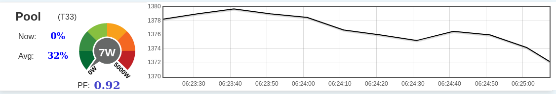
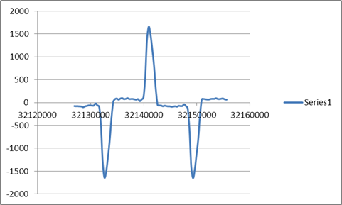
So here is the current profile for my DeWalt battery charger. Once again, I start my sketch with no current running through the wires and then turn the battery charger on. I let it run for a number of seconds before turning it off. My watts-meter gives me a Power Factor of 0.65 for this device.
And here are the measured power numbers out of my six test cases…once again, the first four (taken at widely different sample times) are, for all intents and purposes, identical.
As long as your load is steady, then pretty much any sampling scheme will be accurate over a period of time, with one notable exception of course: if you always sample at the same point or points on each cycle of the wave, you’d better be sure you sample enough points to get a sufficiently accurate representation of the wave.
Let’s construct a silly example to illustrate: If your line frequency is 60 Hz, and you sample at 120 samples/s, then depending on where you start in relation to the wave’s zero crossing, you can read zero on every sample, +max and -max on alternate samples, or anything in between.
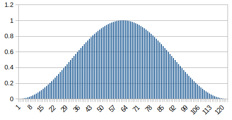
But if you change that to sampling 121 samples/s, you’ll eventually, after a second, get the correct average power. This is what the 121 samples will look like (forget the vertical scale, and it’s a nice well-behaved resistive load): Current: Power:
You must make sure you’re not synchronised with the mains you’re measuring.
Even so, a problem arises when your load isn’t steady. Suppose I turn it off after exactly ¾ second. The average power over the second should be 75%, but it’s clearly not going to be - it’s actually 86% in terms of current, or 91% power. If that’s “good enough”, then fine. But I can’t advocate the method as being generally good and giving accurate answers for everyone, because that’s clearly not the case - as we know from experience with emonLib (the discrete sample version) and loads like induction hobs, where it’s a matter of hit and miss as to whether the heating is on or off when the measurement is taken.
It turns out even ceramic elements are pretty dynamic loads. In this post I reverse engineered the on/off times based on the 10 second true average energy readings.